50K simulations results

Let’s test the 50K simulations results:

from pathlib import Path
from collections import defaultdict

import tskit
import numpy as np
import pandas as pd
import seaborn as sns
import matplotlib.pyplot as plt

from tskitetude import get_project_dir

Let’s declare some stuff

repeats = 5
breed_size = [1, 2, 5, 10, 15, 20]
simulation = "50K_simulations"
reference_prefix = "results-reference"
compara_prefix = "results-compara"
chromosome = "26"

def collect_stats(results_prefix, simulation, chromosome, breed_size, repeats):

    data = defaultdict(list)
    prefix = get_project_dir() / results_prefix / simulation

    for i in breed_size:

        for j in range(repeats):
            run = f"{i}_breeds-{j}-50K"
            filename = prefix / run / "tsinfer" / f"SMARTER-OA-OAR3-forward-0.4.10-50K.focal.{chromosome}.trees"

            if not  filename.exists():
                print(f"File {filename} does not exist")
                continue

            ts = tskit.load(filename)

            # track some stats for tree object
            data["breeds"] += [i]
            data["repeat"] += [j]
            data["filename"] += [filename]
            data["sites"] += [ts.num_sites]
            data["trees"] += [ts.num_trees]
            data["edges"] += [ts.num_edges]
            data["individuals"] += [ts.num_individuals]
            data["samples"] += [ts.num_samples]
            data["mutations"] += [ts.num_mutations]
            data["nodes"] += [ts.num_nodes]
            data["populations"] += [ts.num_populations]

    return pd.DataFrame(data)

Read data from reference simulations:

reference = collect_stats(reference_prefix, simulation, chromosome, breed_size, repeats)
reference.head()

	breeds	repeat	filename	sites	trees	edges	individuals	samples	mutations	nodes	populations
0	1	0	/home/core/TSKITetude/results-reference/50K_si...	792	752	7717	24	48	792	1355	1
1	1	1	/home/core/TSKITetude/results-reference/50K_si...	773	732	7525	24	48	773	1309	1
2	1	2	/home/core/TSKITetude/results-reference/50K_si...	673	616	5974	23	46	673	1102	1
3	1	3	/home/core/TSKITetude/results-reference/50K_si...	766	697	6184	24	48	766	1168	1
4	1	4	/home/core/TSKITetude/results-reference/50K_si...	573	438	3153	21	42	573	707	1

Collect stats for compara:

compara = collect_stats(compara_prefix, simulation, chromosome, breed_size, repeats)
compara.head()

	breeds	repeat	filename	sites	trees	edges	individuals	samples	mutations	nodes	populations
0	1	0	/home/core/TSKITetude/results-compara/50K_simu...	791	557	5667	24	48	1865	1006	1
1	1	1	/home/core/TSKITetude/results-compara/50K_simu...	774	542	5664	24	48	1751	979	1
2	1	2	/home/core/TSKITetude/results-compara/50K_simu...	675	476	4577	23	46	1476	846	1
3	1	3	/home/core/TSKITetude/results-compara/50K_simu...	761	528	4822	24	48	1412	918	1
4	1	4	/home/core/TSKITetude/results-compara/50K_simu...	555	333	2443	21	42	786	553	1

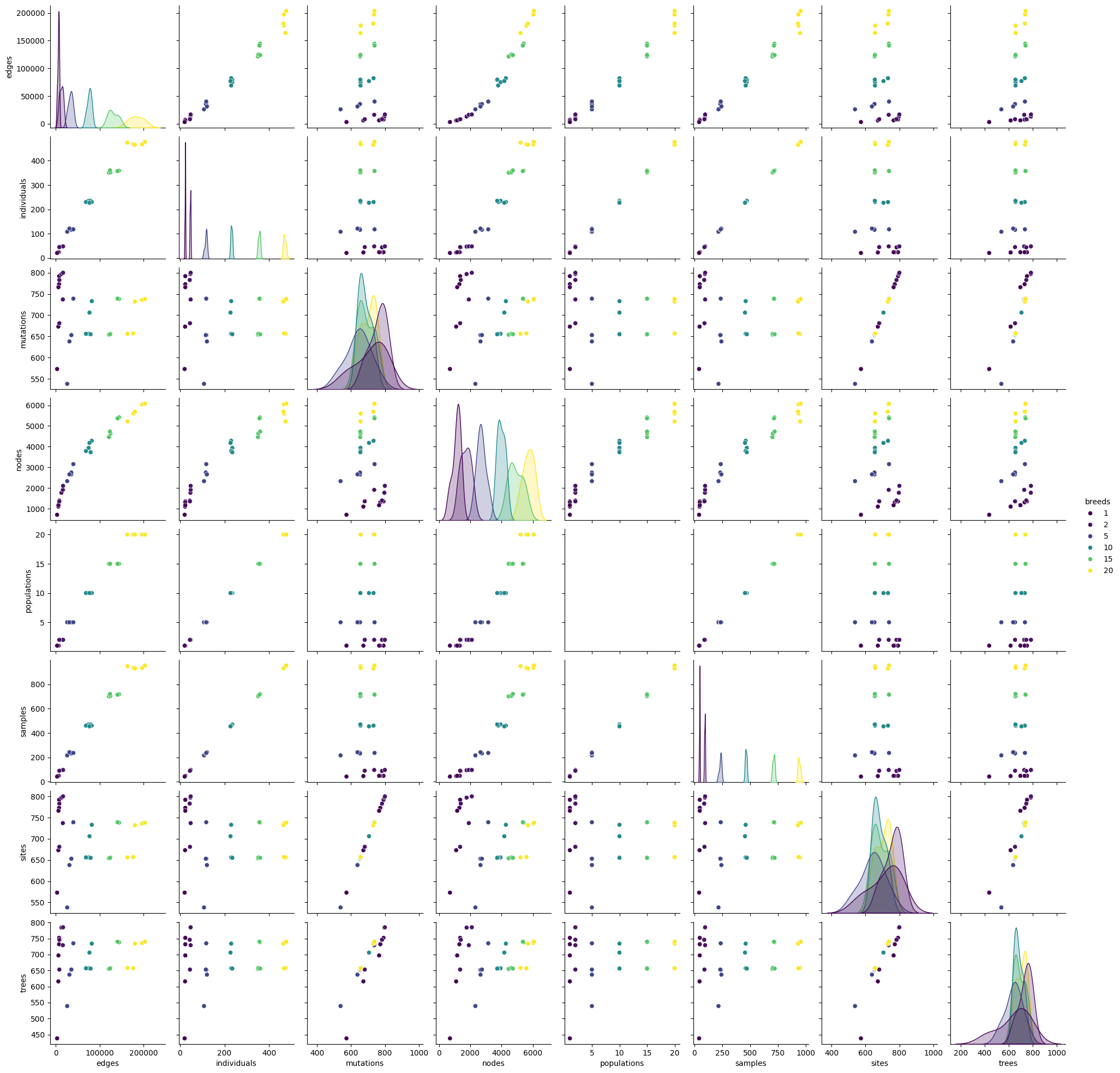
sns.pairplot(reference[reference.columns.difference(['repeat'])], hue="breeds", palette="viridis")

<seaborn.axisgrid.PairGrid at 0x7f66381791c0>

sns.pairplot(compara[compara.columns.difference(["repeat"])], hue="breeds", palette="viridis")

<seaborn.axisgrid.PairGrid at 0x7f65e1f721b0>

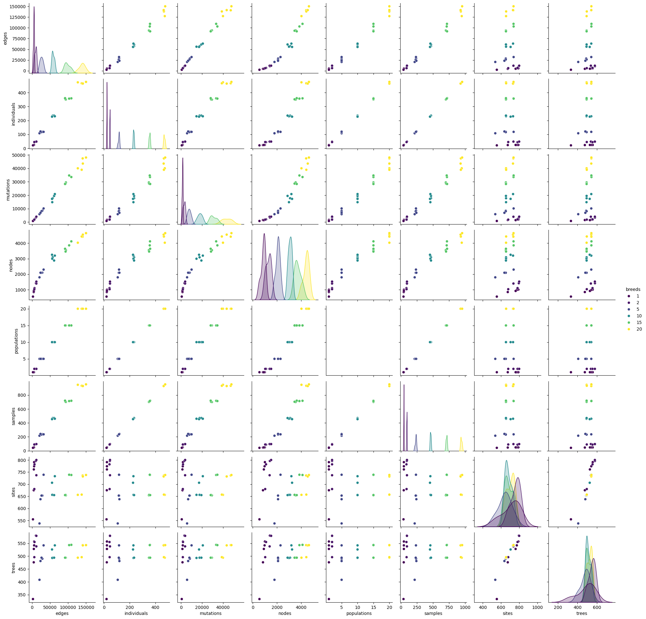
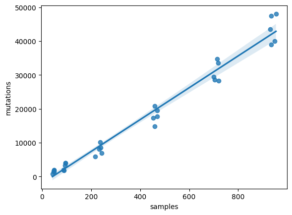
It seems that the number of mutation is higher using the compara approach instead of the reference approach. Let’s try to model the number of mutations relying on the numer or samples. Try to fit a linear model using sns.regplot:

sns.regplot(data=compara, x="samples", y="mutations", ci=95)

<Axes: xlabel='samples', ylabel='mutations'>

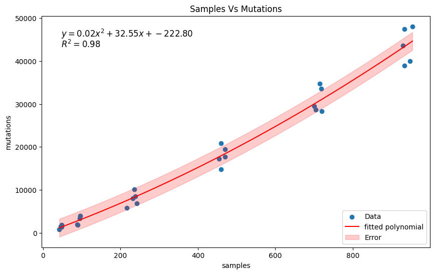
Try to fit a 2nd degree polynomial model using np.polyfit:

# fit a polynomial to the data
coeffs = np.polyfit(compara['samples'], compara['mutations'], 2)
poly = np.poly1d(coeffs)

# generate values for x and y
x_vals = np.linspace(compara['samples'].min(), compara['samples'].max(), 100)
y_vals = poly(x_vals)

# calculate residuals
y_fit = poly(compara['samples'])
residuals = compara['mutations'] - y_fit
std_residuals = np.std(residuals)

# calculate R^2
ss_res = np.sum(residuals**2)
ss_tot = np.sum((compara['mutations'] - np.mean(compara['mutations']))**2)
r2 = 1 - (ss_res / ss_tot)

# plot the data
plt.figure(figsize=(10, 6))
plt.scatter(compara['samples'], compara['mutations'], label='Data')
plt.plot(x_vals, y_vals, color='red', label='fitted polynomial')
plt.fill_between(x_vals, y_vals - std_residuals, y_vals + std_residuals, color='red', alpha=0.2, label='Error')

# add formula to the plot
formula = f'$y = {coeffs[0]:.2f}x^2 + {coeffs[1]:.2f}x + {coeffs[2]:.2f}$'
r2_text = f'$R^2 = {r2:.2f}$'
plt.text(0.05, 0.95, formula, transform=plt.gca().transAxes, fontsize=12, verticalalignment='top')
plt.text(0.05, 0.90, r2_text, transform=plt.gca().transAxes, fontsize=12, verticalalignment='top')

# Add labels and title
plt.xlabel('samples')
plt.ylabel('mutations')
plt.title('Samples Vs Mutations')
plt.legend(loc='lower right')

# Show the plot
plt.show()