Getting started with tskit

This is the step-by-step tutorial found here. Here we generate an alignment using msprime, which is a python package to generate data to be used with tskit stuff

A number of different software programs can generate tree sequences. For the purposes of this tutorial we’ll use msprime to create an example tree sequence representing the genetic genealogy of a 10Mb chromosome in twenty diploid individuals. To make it a bit more interesting, we’ll simulate the effects of a selective sweep in the middle of the chromosome, then throw some neutral mutations onto the resulting tree sequence.

import msprime

pop_size=10_000
seq_length=10_000_000

sweep_model = msprime.SweepGenicSelection(
    position=seq_length/2, start_frequency=0.0001, end_frequency=0.9999, s=0.25, dt=1e-6)

ts = msprime.sim_ancestry(
    20,
    model=[sweep_model, msprime.StandardCoalescent()],
    population_size=pop_size,
    sequence_length=seq_length,
    recombination_rate=1e-8,
    random_seed=1234,  # only needed for repeatabilty
    )
# Optionally add finite-site mutations to the ts using the Jukes & Cantor model, creating SNPs
ts = msprime.sim_mutations(ts, rate=1e-8, random_seed=4321)
ts

Tree Sequence
Trees	11 167
Sequence Length	10 000 000
Time Units	generations
Sample Nodes	40
Total Size	2.4 MiB
Metadata	No Metadata

Table	Rows	Size	Has Metadata
Edges	36 372	1.1 MiB
Individuals	20	584 Bytes
Migrations	0	8 Bytes
Mutations	13 568	490.3 KiB
Nodes	7 342	200.8 KiB
Populations	1	224 Bytes	✅
Provenances	2	1.9 KiB
Sites	13 554	330.9 KiB

Provenance Timestamp	Software Name	Version	Command	Full record
19 December, 2025 at 01:22:45 PM	msprime	1.3.4	sim_mutations	Details dict schema_version: 1.0.0 software: dict name: msprime version: 1.3.4 parameters: dict command: sim_mutations tree_sequence: dict __constant__: __current_ts__ rate: 1e-08 model: None start_time: None end_time: None discrete_genome: None keep: None random_seed: 4321 environment: dict os: dict system: Linux node: node1 release: 5.15.0-58-generic version: #64-Ubuntu SMP Thu Jan 5 11:43:13 UTC 2023 machine: x86_64 python: dict implementation: CPython version: 3.12.12 libraries: dict kastore: dict version: 2.1.1 tskit: dict version: 1.0.0b3 gsl: dict version: 2.6
19 December, 2025 at 01:22:45 PM	msprime	1.3.4	sim_ancestry	Details dict schema_version: 1.0.0 software: dict name: msprime version: 1.3.4 parameters: dict command: sim_ancestry samples: 20 demography: None sequence_length: 10000000 discrete_genome: None recombination_rate: 1e-08 gene_conversion_rate: None gene_conversion_tract_length: None population_size: 10000 ploidy: None model: list dict duration: None position: 5000000.0 start_frequency: 0.0001 end_frequency: 0.9999 s: 0.25 dt: 1e-06 __class__: msprime.ancestry.SweepGenicSel ection dict duration: None __class__: msprime.ancestry.StandardCoale scent initial_state: None start_time: None end_time: None record_migrations: None record_full_arg: None additional_nodes: None coalescing_segments_only: None num_labels: None random_seed: 1234 replicate_index: 0 environment: dict os: dict system: Linux node: node1 release: 5.15.0-58-generic version: #64-Ubuntu SMP Thu Jan 5 11:43:13 UTC 2023 machine: x86_64 python: dict implementation: CPython version: 3.12.12 libraries: dict kastore: dict version: 2.1.1 tskit: dict version: 1.0.0b3 gsl: dict version: 2.6

To cite this software, please consult the citation manual: https://tskit.dev/citation/

We have tousand of trees in ts object. We have 20 dyploid individuals, so 40 nodes (one for genome? have I two genomes per individual as described by the tutorial?)

Processing trees

Iterate over the trees with the trees() method:

for tree in ts.trees():
    print(f"Tree {tree.index} covers {tree.interval}")
    if tree.index >= 4:
        print("...")
        break
print(f"Tree {ts.last().index} covers {ts.last().interval}")

Tree 0 covers Interval(left=0.0, right=661.0)
Tree 1 covers Interval(left=661.0, right=3116.0)
Tree 2 covers Interval(left=3116.0, right=4451.0)
Tree 3 covers Interval(left=4451.0, right=4673.0)
Tree 4 covers Interval(left=4673.0, right=5020.0)
...
Tree 11166 covers Interval(left=9999635.0, right=10000000.0)

There are also last() and first() methods to access to the last and first trees respectively. Check if trees coalesce (not always true for forward simulations)

import time
elapsed = time.time()
for tree in ts.trees():
    if tree.has_multiple_roots:
        print("Tree {tree.index} has not coalesced")
        break
else:
    elapsed = time.time() - elapsed
    print(f"All {ts.num_trees} trees coalesced")
    print(f"Checked in {elapsed:.6g} secs")

All 11167 trees coalesced
Checked in 0.0111287 secs

Now that we know all trees have coalesced, we know that at each position in the genome all the 40 sample nodes must have one most recent common ancestor (MRCA). Below, we iterate over the trees, finding the IDs of the root (MRCA) node for e ach tree. The time of this root node can be found via the tskit.TreeSequence.node() method, which returns a Node object whose attributes include the node time:

import matplotlib.pyplot as plt

kb = [0]  # Starting genomic position
mrca_time = []
for tree in ts.trees():
    kb.append(tree.interval.right/1000)  # convert to kb
    mrca = ts.node(tree.root)  # For msprime tree sequences, the root node is the MRCA
    mrca_time.append(mrca.time)
plt.stairs(mrca_time, kb, baseline=None)
plt.xlabel("Genome position (kb)")
plt.ylabel("Time of root (or MRCA) in generations")
plt.yscale("log")
plt.show()

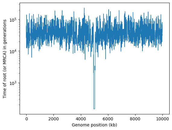
It’s obvious that there’s something unusual about the trees in the middle of this chromosome, where the selective sweep occurred.

Although tskit is designed so that is it rapid to pass through trees sequentially, it is also possible to pull out individual trees from the middle of a tree sequence via the TreeSequence.at() method. Here’s how you can use that to extract the tree at location - the position of the sweep - and draw it using the Tree.draw_svg() method:

swept_tree = ts.at(5_000_000)  # or you can get e.g. the nth tree using ts.at_index(n)
intvl = swept_tree.interval
print(f"Tree number {swept_tree.index}, which runs from position {intvl.left} to {intvl.right}:")
# Draw it at a wide size, to make room for all 40 tips
swept_tree.draw_svg(size=(1000, 200))

Tree number 5382, which runs from position 4998293.0 to 5033047.0:

This tree shows the classic signature of a recent expansion or selection event, with many long terminal branches, resulting in an excess of singleton mutations.

It can often be helpful to slim down a tree sequence so that it represents the genealogy of a smaller subset of the original samples. This can be done using the powerful TreeSequence.simplify() method.

The TreeSequence.draw_svg() method allows us to draw more than one tree: either the entire tree sequence, or (by using the x_lim parameter) a smaller region of the genome:

reduced_ts = ts.simplify([0, 1, 2, 3, 4, 5, 6, 7, 8, 9])  # simplify to the first 10 samples
print("Genealogy of the first 10 samples for the first 5kb of the genome")
reduced_ts.draw_svg(x_lim=(0, 5000))

Genealogy of the first 10 samples for the first 5kb of the genome

These are much more standard-looking coalescent trees, with far longer branches higher up in the tree, and therefore many more mutations at higher-frequencies.

In this tutorial we refer to objects, such as sample nodes, by their numerical IDs. These can change after simplification, and it is often more meaningful to work with metadata, such as sample and population names, which can be permanently attached to objects in the tree sequence. Such metadata is often incorporated automatically by the tools generating the tree sequence.

Processing sites and mutations

For many purposes it may be better to focus on the genealogy of your samples, rather than the sites and mutations that define the genome sequence itself. Nevertheless, tskit also provides efficient ways to return Site object and Mutation objects from a tree sequence. For instance, under the finite sites model of mutation that we used above, multiple mutations can occur at some sites, and we can identify them by iterating over the sites using the TreeSequence.sites() method:

import numpy as np

num_muts = np.zeros(ts.num_sites, dtype=int)

for site in ts.sites():
    num_muts[site.id] = len(site.mutations)  # site.mutations is a list of mutations at the site

# Print out some info about mutations per site
for nmuts, count in enumerate(np.bincount(num_muts)):
    info = f"{count} sites"
    if nmuts > 1:
        info += f", with IDs {np.where(num_muts==nmuts)[0]},"
    print(info, f"have {nmuts} mutation" + ("s" if nmuts != 1 else ""))

0 sites have 0 mutations
13540 sites have 1 mutation
14 sites, with IDs [ 2275  2287  2658  3789  4043  9694 11023 11780 11853 11890 11999 12023
 12096 12310], have 2 mutations

Processing genotypes

At each site, the sample nodes will have a particular allelic state (or be flagged as Missing data). The TreeSequence.variants() method gives access to the full variation data. For efficiency, the genotypes at a site are returned as a numpy array of integers:

np.set_printoptions(linewidth=200)  # print genotypes on a single line

print("Genotypes")
for v in ts.variants():
    print(f"Site {v.site.id}: {v.genotypes}")
    if v.site.id >= 4:  # only print up to site ID 4
        print("...")
        break

Genotypes
Site 0: [0 0 1 1 0 0 1 0 0 0 0 0 0 0 1 0 0 0 0 0 0 0 0 1 0 0 1 0 0 0 0 0 1 0 1 0 0 0 0 0]
Site 1: [1 1 0 0 1 1 0 1 1 1 1 1 1 1 0 1 1 1 1 1 1 1 1 0 0 1 0 1 1 1 1 1 0 1 0 1 0 0 1 1]
Site 2: [0 0 1 1 0 0 1 0 0 0 0 0 0 0 1 0 0 0 0 0 0 0 0 1 0 0 1 0 0 0 0 0 1 0 1 0 0 0 0 0]
Site 3: [0 0 0 0 0 0 0 0 0 0 0 0 0 0 1 0 0 0 0 0 0 0 0 0 0 0 0 0 0 0 0 0 0 0 0 0 0 0 0 0]
Site 4: [0 0 1 1 0 0 1 0 0 0 0 0 0 0 1 0 0 0 0 0 0 0 0 1 0 0 1 0 0 0 0 0 1 0 1 0 0 0 0 0]
...

Tree sequences are optimised to look at all samples at one site, then all samples at an adjacent site, and so on along the genome. It is much less efficient look at all the sites for a single sample, then all the sites for the next sample, etc. In other words, you should generally iterate over sites, not samples. Nevertheless, all the alleles for a single sample can be obtained via the TreeSequence.haplotypes() method.

To find the actual allelic states at a site, you can refer to the alleles provided for each Variant: the genotype value is an index into this list. Here’s one way to print them out; for clarity this example also prints out the IDs of both the sample nodes (i.e. the genomes) and the diploid individuals in which each sample node resides.

samp_ids = ts.samples()

print("  ID of diploid individual: ", " ".join([f"{ts.node(s).individual:3}" for s in samp_ids]))
print("       ID of (sample) node: ", " ".join([f"{s:3}" for s in samp_ids]))

for v in ts.variants():
    site = v.site
    alleles = np.array(v.alleles)
    print(f"Site {site.id} (ancestral state '{site.ancestral_state}')",  alleles[v.genotypes])
    if site.id >= 4:  # only print up to site ID 4
        print("...")
        break

  ID of diploid individual:    0   0   1   1   2   2   3   3   4   4   5   5   6   6   7   7   8   8   9   9  10  10  11  11  12  12  13  13  14  14  15  15  16  16  17  17  18  18  19  19
       ID of (sample) node:    0   1   2   3   4   5   6   7   8   9  10  11  12  13  14  15  16  17  18  19  20  21  22  23  24  25  26  27  28  29  30  31  32  33  34  35  36  37  38  39
Site 0 (ancestral state 'G') ['G' 'G' 'T' 'T' 'G' 'G' 'T' 'G' 'G' 'G' 'G' 'G' 'G' 'G' 'T' 'G' 'G' 'G' 'G' 'G' 'G' 'G' 'G' 'T' 'G' 'G' 'T' 'G' 'G' 'G' 'G' 'G' 'T' 'G' 'T' 'G' 'G' 'G' 'G' 'G']
Site 1 (ancestral state 'T') ['G' 'G' 'T' 'T' 'G' 'G' 'T' 'G' 'G' 'G' 'G' 'G' 'G' 'G' 'T' 'G' 'G' 'G' 'G' 'G' 'G' 'G' 'G' 'T' 'T' 'G' 'T' 'G' 'G' 'G' 'G' 'G' 'T' 'G' 'T' 'G' 'T' 'T' 'G' 'G']
Site 2 (ancestral state 'T') ['T' 'T' 'C' 'C' 'T' 'T' 'C' 'T' 'T' 'T' 'T' 'T' 'T' 'T' 'C' 'T' 'T' 'T' 'T' 'T' 'T' 'T' 'T' 'C' 'T' 'T' 'C' 'T' 'T' 'T' 'T' 'T' 'C' 'T' 'C' 'T' 'T' 'T' 'T' 'T']
Site 3 (ancestral state 'T') ['T' 'T' 'T' 'T' 'T' 'T' 'T' 'T' 'T' 'T' 'T' 'T' 'T' 'T' 'A' 'T' 'T' 'T' 'T' 'T' 'T' 'T' 'T' 'T' 'T' 'T' 'T' 'T' 'T' 'T' 'T' 'T' 'T' 'T' 'T' 'T' 'T' 'T' 'T' 'T']
Site 4 (ancestral state 'T') ['T' 'T' 'A' 'A' 'T' 'T' 'A' 'T' 'T' 'T' 'T' 'T' 'T' 'T' 'A' 'T' 'T' 'T' 'T' 'T' 'T' 'T' 'T' 'A' 'T' 'T' 'A' 'T' 'T' 'T' 'T' 'T' 'A' 'T' 'A' 'T' 'T' 'T' 'T' 'T']
...