Reading data from chromosome 26#
This notebook demonstrates how to read data from TreeSequence objects and perform some basic statistics on the data. We will use the chromosome 26 data from the SMARTER background dataset, calculated with the compara approach
import tskit
import tsinfer
import numpy as np
import pandas as pd
import matplotlib.pyplot as plt

from tskitetude import get_project_dir
loading data from one chromosome:
ts = tskit.load(get_project_dir() / "results-compara/background_samples/tsinfer/SMARTER-OA-OAR3-forward-0.4.10.focal.26.trees")
ts
|
|
|
|---|---|
| Trees | 496 |
| Sequence Length | 44 077 779 |
| Time Units | generations |
| Sample Nodes | 11 478 |
| Total Size | 89.9 MiB |
| Metadata |
dict |
| Table | Rows | Size | Has Metadata |
|---|---|---|---|
| Edges | 1 838 362 | 56.1 MiB | |
| Individuals | 5 739 | 353.1 KiB | ✅ |
| Migrations | 0 | 8 Bytes | |
| Mutations | 524 747 | 18.5 MiB | |
| Nodes | 19 188 | 932.4 KiB | ✅ |
| Populations | 202 | 4.7 KiB | ✅ |
| Provenances | 4 | 2.4 KiB | |
| Sites | 657 | 33.5 KiB | ✅ |
| Provenance Timestamp | Software Name | Version | Command | Full record |
|---|---|---|---|---|
| 06 September, 2024 at 02:30:20 AM | tsdate | 0.1.7 | inside_outside |
Detailsdictschema_version: 1.0.0
software:
dictname: tsdateversion: 0.1.7
parameters:
dictmutation_rate: 1e-08recombination_rate: None time_units: None progress: None population_size: 10000.0 eps: 1e-06 outside_standardize: True ignore_oldest_root: False probability_space: logarithmic num_threads: None cache_inside: False command: inside_outside
environment:
dict
os:
dictsystem: Linuxnode: node1 release: 5.15.0-58-generic version: #64-Ubuntu SMP Thu Jan 5 11:43:13 UTC 2023 machine: x86_64
python:
dictimplementation: CPythonversion: 3.11.9
libraries:
dict
tskit:
dictversion: 0.5.8 |
| 06 September, 2024 at 02:25:05 AM | tsdate | 0.1.7 | preprocess_ts |
Detailsdictschema_version: 1.0.0
software:
dictname: tsdateversion: 0.1.7
parameters:
dictminimum_gap: 1000000remove_telomeres: True filter_populations: False filter_individuals: False filter_sites: False
delete_intervals:
listlist0209048.0 list44004282.044077779.0 command: preprocess_ts
environment:
dict
os:
dictsystem: Linuxnode: node1 release: 5.15.0-58-generic version: #64-Ubuntu SMP Thu Jan 5 11:43:13 UTC 2023 machine: x86_64
python:
dictimplementation: CPythonversion: 3.11.9
libraries:
dict
tskit:
dictversion: 0.5.8 |
| 06 September, 2024 at 02:25:01 AM | tskit | 0.5.8 | simplify |
Detailsdictschema_version: 1.0.0
software:
dictname: tskitversion: 0.5.8
parameters:
dictcommand: simplifyTODO: add simplify parameters
environment:
dict
os:
dictsystem: Linuxnode: node1 release: 5.15.0-58-generic version: #64-Ubuntu SMP Thu Jan 5 11:43:13 UTC 2023 machine: x86_64
python:
dictimplementation: CPythonversion: 3.11.9
libraries:
dict
kastore:
dictversion: 2.1.1 |
| 06 September, 2024 at 02:25:00 AM | tsinfer | 0.3.3 | infer |
Detailsdictschema_version: 1.0.0
software:
dictname: tsinferversion: 0.3.3
parameters:
dictmismatch_ratio: Nonecommand: infer
environment:
dict
libraries:
dict
zarr:
dictversion: 2.17.2
numcodecs:
dictversion: 0.12.1
lmdb:
dictversion: 1.4.1
tskit:
dictversion: 0.5.8
os:
dictsystem: Linuxnode: node1 release: 5.15.0-58-generic version: #64-Ubuntu SMP Thu Jan 5 11:43:13 UTC 2023 machine: x86_64
python:
dictimplementation: CPython
version:
list311 9 |
samples = tsinfer.load(get_project_dir() / "results-compara/background_samples/tsinfer/SMARTER-OA-OAR3-forward-0.4.10.focal.26.samples")
print(samples.info)
Name        : /
Type        : zarr.hierarchy.Group
Read-only   : True
Store type  : zarr.storage.LMDBStore
No. members : 5
No. arrays  : 0
No. groups  : 5
Groups      : individuals, populations, provenances, samples, sites
--------------------------------------------------------------------------------
Name               : /individuals/flags
Type               : zarr.core.Array
Data type          : uint32
Shape              : (5739,)
Chunk shape        : (1024,)
Order              : C
Read-only          : True
Compressor         : Zstd(level=1)
Store type         : zarr.storage.LMDBStore
No. bytes          : 22956 (22.4K)
No. bytes stored   : 389
Storage ratio      : 59.0
Chunks initialized : 6/6
--------------------------------------------------------------------------------
Name               : /individuals/location
Type               : zarr.core.Array
Data type          : object
Shape              : (5739,)
Chunk shape        : (1024,)
Order              : C
Read-only          : True
Filter [0]         : VLenArray(dtype='<f8')
Compressor         : Zstd(level=1)
Store type         : zarr.storage.LMDBStore
No. bytes          : 45912 (44.8K)
No. bytes stored   : 656
Storage ratio      : 70.0
Chunks initialized : 6/6
--------------------------------------------------------------------------------
Name               : /individuals/metadata
Type               : zarr.core.Array
Data type          : object
Shape              : (5739,)
Chunk shape        : (1024,)
Order              : C
Read-only          : True
Filter [0]         : JSON(encoding='utf-8', allow_nan=True, check_circular=True,
                   : ensure_ascii=True,      indent=None, separators=(',', ':'),
                   : skipkeys=False, sort_keys=True,      strict=True)
Compressor         : Zstd(level=1)
Store type         : zarr.storage.LMDBStore
No. bytes          : 45912 (44.8K)
No. bytes stored   : 8621 (8.4K)
Storage ratio      : 5.3
Chunks initialized : 6/6
--------------------------------------------------------------------------------
Name               : /individuals/population
Type               : zarr.core.Array
Data type          : int32
Shape              : (5739,)
Chunk shape        : (1024,)
Order              : C
Read-only          : True
Compressor         : Zstd(level=1)
Store type         : zarr.storage.LMDBStore
No. bytes          : 22956 (22.4K)
No. bytes stored   : 1270 (1.2K)
Storage ratio      : 18.1
Chunks initialized : 6/6
--------------------------------------------------------------------------------
Name               : /individuals/time
Type               : zarr.core.Array
Data type          : float64
Shape              : (5739,)
Chunk shape        : (1024,)
Order              : C
Read-only          : True
Compressor         : Zstd(level=1)
Store type         : zarr.storage.LMDBStore
No. bytes          : 45912 (44.8K)
No. bytes stored   : 391
Storage ratio      : 117.4
Chunks initialized : 6/6
--------------------------------------------------------------------------------
Name               : /populations/metadata
Type               : zarr.core.Array
Data type          : object
Shape              : (202,)
Chunk shape        : (1024,)
Order              : C
Read-only          : True
Filter [0]         : JSON(encoding='utf-8', allow_nan=True, check_circular=True,
                   : ensure_ascii=True,      indent=None, separators=(',', ':'),
                   : skipkeys=False, sort_keys=True,      strict=True)
Compressor         : Zstd(level=1)
Store type         : zarr.storage.LMDBStore
No. bytes          : 1616 (1.6K)
No. bytes stored   : 1191 (1.2K)
Storage ratio      : 1.4
Chunks initialized : 1/1
--------------------------------------------------------------------------------
Name               : /provenances/record
Type               : zarr.core.Array
Data type          : object
Shape              : (0,)
Chunk shape        : (1024,)
Order              : C
Read-only          : True
Filter [0]         : JSON(encoding='utf-8', allow_nan=True, check_circular=True,
                   : ensure_ascii=True,      indent=None, separators=(',', ':'),
                   : skipkeys=False, sort_keys=True,      strict=True)
Compressor         : Zstd(level=1)
Store type         : zarr.storage.LMDBStore
No. bytes          : 0
No. bytes stored   : 624
Storage ratio      : 0.0
Chunks initialized : 0/0
--------------------------------------------------------------------------------
Name               : /provenances/timestamp
Type               : zarr.core.Array
Data type          : object
Shape              : (0,)
Chunk shape        : (1024,)
Order              : C
Read-only          : True
Filter [0]         : JSON(encoding='utf-8', allow_nan=True, check_circular=True,
                   : ensure_ascii=True,      indent=None, separators=(',', ':'),
                   : skipkeys=False, sort_keys=True,      strict=True)
Compressor         : Zstd(level=1)
Store type         : zarr.storage.LMDBStore
No. bytes          : 0
No. bytes stored   : 624
Storage ratio      : 0.0
Chunks initialized : 0/0
--------------------------------------------------------------------------------
Name               : /samples/individual
Type               : zarr.core.Array
Data type          : int32
Shape              : (11478,)
Chunk shape        : (1024,)
Order              : C
Read-only          : True
Compressor         : Zstd(level=1)
Store type         : zarr.storage.LMDBStore
No. bytes          : 45912 (44.8K)
No. bytes stored   : 6630 (6.5K)
Storage ratio      : 6.9
Chunks initialized : 12/12
--------------------------------------------------------------------------------
Name               : /sites/alleles
Type               : zarr.core.Array
Data type          : object
Shape              : (657,)
Chunk shape        : (1024,)
Order              : C
Read-only          : True
Filter [0]         : JSON(encoding='utf-8', allow_nan=True, check_circular=True,
                   : ensure_ascii=True,      indent=None, separators=(',', ':'),
                   : skipkeys=False, sort_keys=True,      strict=True)
Compressor         : Zstd(level=1)
Store type         : zarr.storage.LMDBStore
No. bytes          : 5256 (5.1K)
No. bytes stored   : 1455 (1.4K)
Storage ratio      : 3.6
Chunks initialized : 1/1
--------------------------------------------------------------------------------
Name               : /sites/ancestral_allele
Type               : zarr.core.Array
Data type          : int8
Shape              : (657,)
Chunk shape        : (1024,)
Order              : C
Read-only          : True
Compressor         : Zstd(level=1)
Store type         : zarr.storage.LMDBStore
No. bytes          : 657
No. bytes stored   : 489
Storage ratio      : 1.3
Chunks initialized : 1/1
--------------------------------------------------------------------------------
Name               : /sites/genotypes
Type               : zarr.core.Array
Data type          : int8
Shape              : (657, 11478)
Chunk shape        : (1024, 1024)
Order              : C
Read-only          : True
Compressor         : Zstd(level=1)
Store type         : zarr.storage.LMDBStore
No. bytes          : 7541046 (7.2M)
No. bytes stored   : 1305890 (1.2M)
Storage ratio      : 5.8
Chunks initialized : 12/12
--------------------------------------------------------------------------------
Name               : /sites/metadata
Type               : zarr.core.Array
Data type          : object
Shape              : (657,)
Chunk shape        : (1024,)
Order              : C
Read-only          : True
Filter [0]         : JSON(encoding='utf-8', allow_nan=True, check_circular=True,
                   : ensure_ascii=True,      indent=None, separators=(',', ':'),
                   : skipkeys=False, sort_keys=True,      strict=True)
Compressor         : Zstd(level=1)
Store type         : zarr.storage.LMDBStore
No. bytes          : 5256 (5.1K)
No. bytes stored   : 696
Storage ratio      : 7.6
Chunks initialized : 1/1
--------------------------------------------------------------------------------
Name               : /sites/position
Type               : zarr.core.Array
Data type          : float64
Shape              : (657,)
Chunk shape        : (1024,)
Order              : C
Read-only          : True
Compressor         : Zstd(level=1)
Store type         : zarr.storage.LMDBStore
No. bytes          : 5256 (5.1K)
No. bytes stored   : 2420 (2.4K)
Storage ratio      : 2.2
Chunks initialized : 1/1
--------------------------------------------------------------------------------
Name               : /sites/time
Type               : zarr.core.Array
Data type          : float64
Shape              : (657,)
Chunk shape        : (1024,)
Order              : C
Read-only          : True
Compressor         : Zstd(level=1)
Store type         : zarr.storage.LMDBStore
No. bytes          : 5256 (5.1K)
No. bytes stored   : 306
Storage ratio      : 17.2
Chunks initialized : 1/1
/home/cozzip/.cache/pypoetry/virtualenvs/tskitetude-hh-GIRXc-py3.12/lib/python3.12/site-packages/tsinfer/formats.py:104: FutureWarning: The LMDBStore is deprecated and will be removed in a Zarr-Python version 3, see https://github.com/zarr-developers/zarr-python/issues/1274 for more information.
  store = zarr.LMDBStore(
Displaying data#
The first thing I see that was different from tutorial is that the first tree looks a lot different from the second:
first = ts.first()
second = ts.at_index(1)
first
|
|
|
|---|---|
| Index | 0 |
| Interval | 0-209 049 (209 049) |
| Roots | 11 478 |
| Nodes | 11 478 |
| Sites | 0 |
| Mutations | 0 |
| Total Branch Length | 0 |
second
|
|
|
|---|---|
| Index | 1 |
| Interval | 209 049-268 822 (59 773) |
| Roots | 1 |
| Nodes | 11 530 |
| Sites | 1 |
| Mutations | 1 |
| Total Branch Length | 1 513 559.3 |
Try to modify visualization tutorial to display the second tree:
x_limits = [int(second.interval[0]), int(second.interval[1])]

# Create evenly-spaced y tick positions to avoid overlap
# y_tick_pos = [0, 1000, 2000, 3000, 4000]
y_tick_pos = np.linspace(0, second.span, num=int(second.span / 10_000))

print("The tree sequence between positions {} and {} ...".format(*x_limits))

# this is a single tree, not a tree sequence (see: https://tskit.dev/tskit/docs/stable/python-api.html#tskit.Tree.draw_svg)
display(
    second.draw_svg(
        y_axis=True,
        y_ticks=y_tick_pos,
        size=(1024, 768),
        time_scale="log_time",
    )
)
WARNING:root:Ticks {np.float64(14943.25): '14943.25', np.float64(29886.5): '29886.50', np.float64(44829.75): '44829.75', np.float64(59773.0): '59773.00'} lie outside the plotted axis
The tree sequence between positions 209049 and 268822 ...

print("A larger tree, on a log timescale")
wide_fmt = (250000, 2000)

# Create a stylesheet that shrinks labels and rotates leaf labels, to avoid overlap
node_label_style = (
    ".node > .lab {font-size: 80%}"
    ".leaf > .lab {text-anchor: start; transform: rotate(90deg) translate(6px)}"
)
second.draw_svg(
    size=wide_fmt,
    time_scale="log_time",
    y_gridlines=True,
    y_axis=True,
    y_ticks=[1, 10, 100, 1000],
    style=node_label_style,
)
WARNING:root:Ticks {1000: '1000'} lie outside the plotted axis
A larger tree, on a log timescale

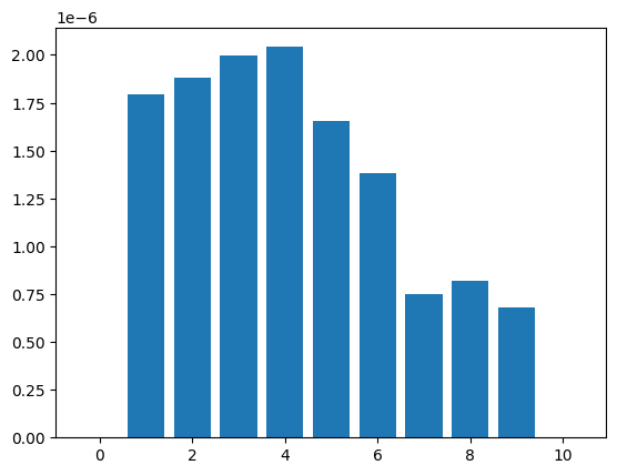
site-frequency spectrum#
Calculate site-frequency spectrum:
plt.bar(np.array(range(11)), ts.simplify(range(10)).allele_frequency_spectrum(polarised=True, span_normalise=True))
plt.show()
One-way statistics#
We refer to statistics that are defined with respect to a single set of samples as “one-way”. An example of such a statistic is diversity, which is computed using the TreeSequence.diversity() method:
pi = ts.diversity()
print(f"Average diversity per unit sequence length = {pi:.3G}")
Average diversity per unit sequence length = 5.96E-06
Computes mean genetic diversity (also known as pi) in each of the sets of nodes from sample_sets. The statistic is also known as sample heterozygosity; a common citation for the definition is Nei and Li (1979) (equation 22), so it is sometimes called called “Nei’s pi” (but also sometimes “Tajima’s pi”). This tells the average diversity across the whole sequence and returns a single number. We’ll usually want to compute statistics in windows along the genome and we use the windows argument to do this:
print("Sequence length = ", ts.sequence_length)
# windows = np.linspace(0, ts.sequence_length, num=int(ts.sequence_length / 1_000_000) + 1)
# it's seems that windows needs to contain the initial and final positions
windows = np.append(np.arange(0, ts.sequence_length, 5_000_000), ts.sequence_length)
# transform into integer
windows = windows.astype(int)
pi = ts.diversity(windows=windows)
df = pd.DataFrame({"windows": windows[1:], "pi": pi})
df["pi"] = df["pi"].map(lambda x: f"{x:.3G}")
df
Sequence length = 44077779.0
| windows | pi | |
|---|---|---|
| 0 | 5000000 | 6.08E-06 |
| 1 | 10000000 | 5.5E-06 |
| 2 | 15000000 | 5.55E-06 |
| 3 | 20000000 | 5.94E-06 |
| 4 | 25000000 | 6E-06 |
| 5 | 30000000 | 6.54E-06 |
| 6 | 35000000 | 5.27E-06 |
| 7 | 40000000 | 6.08E-06 |
| 8 | 44077779 | 6.86E-06 |
Suppose we wanted to compute diversity within a specific subset of samples. We can do this using the sample_sets argument:
A = ts.samples()[:100]
d = ts.diversity(sample_sets=A)
print(d)
5.692838488247723e-06
Here, we’ve computed the average diversity within the first hundred samples across the whole genome. As we’ve not specified any windows, this is again a single value. We can also compute diversity in multiple sample sets at the same time by providing a list of sample sets as an argument:
A = ts.samples()[:100]
B = ts.samples()[100:200]
C = ts.samples()[200:300]
d = ts.diversity(sample_sets=[A, B, C])
print(d)
[5.69283849e-06 5.64950370e-06 5.67518833e-06]
Ok, this was done by following the tutorial an getting samples by indexes. But can I select my data by breeds? this information seems not to be stored in tstree object itself, but in the sample data I used to generate my stuff. Let’s discover the samples by breed. Remember that in my data I have 11477 samples, which stand for a pair of chromosomes for my 5739 individuals:
print(f"I have {ts.samples().size} samples")
print(f"which stand for {sum(1 for _ in samples.individuals())} individuals")
I have 11478 samples
which stand for 5739 individuals
def get_sample_indexes(samples: tsinfer.SampleData, breed: str):
    # return np.where(samples.individuals_metadata["breed"] == breed)[0]
    # get breed index from samples.population_metadata
    breed_idx = next((index for index, d in enumerate(samples.populations_metadata) if d['breed'] == breed), None)

    # get individuals indexes by breed index
    individuals = [i.id for i in filter(lambda i: i.population == breed_idx, samples.individuals())]

    # get samples by individual index
    samples = [s.id for s in filter(lambda s: s.individual in individuals, samples.samples())]

    return samples
Get indexes for MER and TEX and calculate diversity:
TEX = get_sample_indexes(samples, "TEX")
MER = get_sample_indexes(samples, "MER")
pi = ts.diversity(sample_sets=[TEX, MER])
print(pi)
[5.83822688e-06 5.82979559e-06]
Same stuff as before but using windows:
windows = np.append(np.arange(0, ts.sequence_length, 5_000_000), ts.sequence_length)
windows = windows.astype(int)
pi = ts.diversity(sample_sets=[TEX, MER], windows=windows)
df = pd.DataFrame({"windows": windows[1:], "MER_pi": pi[:, 0], "TEX_pi": pi[:, 1]})
df["MER_pi"] = df["MER_pi"].map(lambda x: f"{x:.3G}")
df["TEX_pi"] = df["TEX_pi"].map(lambda x: f"{x:.3G}")
df
| windows | MER_pi | TEX_pi | |
|---|---|---|---|
| 0 | 5000000 | 6.09E-06 | 6.12E-06 |
| 1 | 10000000 | 5.38E-06 | 5.37E-06 |
| 2 | 15000000 | 5.49E-06 | 5.35E-06 |
| 3 | 20000000 | 5.55E-06 | 5.74E-06 |
| 4 | 25000000 | 5.94E-06 | 5.88E-06 |
| 5 | 30000000 | 6.28E-06 | 6.39E-06 |
| 6 | 35000000 | 5.26E-06 | 5.28E-06 |
| 7 | 40000000 | 5.99E-06 | 5.91E-06 |
| 8 | 44077779 | 6.72E-06 | 6.54E-06 |
Multi-way statistics#
Many population genetic statistics compare multiple sets of samples to each other. For example, the TreeSequence.divergence() method computes the divergence between two subsets of samples:
d = ts.divergence([TEX, MER])
print(f"Divergence between TEX and MER: {d:.3G}")
Divergence between TEX and MER: 5.95E-06
The divergence between two sets of samples is a single number, and we we again return a single floating point value as the result. We can also compute this in windows along the genome, as before:
d = ts.divergence([TEX, MER], windows=windows)
print(d)
[6.21551166e-06 5.47266300e-06 5.56901446e-06 5.76647237e-06
 6.07222582e-06 6.44783571e-06 5.35874352e-06 6.06778929e-06
 6.77429612e-06]
A powerful feature of tskit’s stats API is that we can compute the divergences between multiple sets of samples simultaneously using the indexes argument:
CRL = get_sample_indexes(samples, "CRL")
d = ts.divergence([TEX, MER, CRL], indexes=[(0, 1), (0, 2)])
print(d)
[5.95482276e-06 5.96852516e-06]
The indexes argument is used to specify which pairs of sets we are interested in. In this example we’ve computed two different divergence values and the output is therefore a numpy array of length 2.
As before, we can combine computing multiple statistics in multiple windows to return a 2D numpy array:
d = ts.divergence([TEX, MER, CRL], indexes=[(0, 1), (0, 2)], windows=windows)
df = pd.DataFrame({"windows": windows[1:], "TEXvsMER": d[:, 0], "MERvsCRL": d[:, 1]})
for column in df.columns[1:]:
    df[column] = df[column].map(lambda x: f"{x:.3G}")
df
| windows | TEXvsMER | MERvsCRL | |
|---|---|---|---|
| 0 | 5000000 | 6.22E-06 | 6.21E-06 |
| 1 | 10000000 | 5.47E-06 | 5.54E-06 |
| 2 | 15000000 | 5.57E-06 | 5.63E-06 |
| 3 | 20000000 | 5.77E-06 | 5.64E-06 |
| 4 | 25000000 | 6.07E-06 | 6.01E-06 |
| 5 | 30000000 | 6.45E-06 | 6.47E-06 |
| 6 | 35000000 | 5.36E-06 | 5.44E-06 |
| 7 | 40000000 | 6.07E-06 | 6.09E-06 |
| 8 | 44077779 | 6.77E-06 | 6.84E-06 |
Each row again corresponds to a window, which contains the average divergence values between the chosen sets.